
How to Find Missing Values in Two Excel Worksheets


Using the VLOOKUP Function
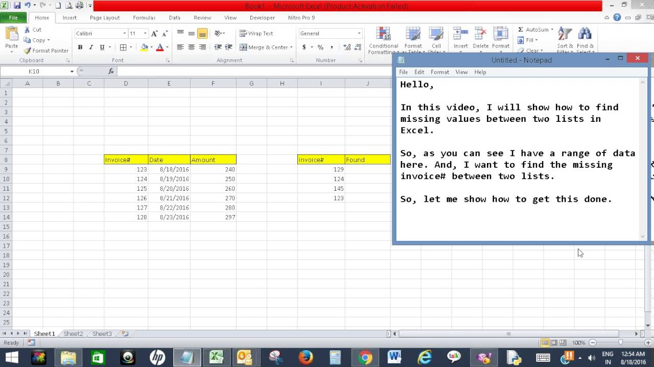
When working with large datasets in Excel, it's common to encounter missing values. Finding these missing values, especially when comparing two worksheets, can be a challenging task. However, with the right techniques, you can easily identify and manage missing data in your Excel spreadsheets. In this article, we'll explore the simple steps to find missing values in two Excel worksheets.
To find missing values in two worksheets, you can use the VLOOKUP function or conditional formatting. The VLOOKUP function allows you to search for a value in a table and return a corresponding value from another column. By using this function, you can compare the data in two worksheets and identify missing values. On the other hand, conditional formatting enables you to highlight cells that meet specific conditions, making it easier to spot missing values.
Using Conditional Formatting
The VLOOKUP function is a powerful tool in Excel that can help you find missing values in two worksheets. To use this function, simply enter the formula =VLOOKUP(lookup value, table array, col index num, [range lookup]) in the cell where you want to display the result. The lookup value is the value you want to search for, the table array is the range of cells that contains the data you want to search, and the col index num is the column number that contains the value you want to return. By using this function, you can quickly identify missing values in your data.